Rotor Average Models

The rotor average model in PyWake defines one or more points at the turbine rotor to calculate a (weighted) rotor-average deficit. It includes:

• RotorCenter: One point at the center of the rotor

• GridRotorAvg: Custom grid in Cartesian coordinates’

• EqGridRotorAvg: Equidistant N x N Cartesian grid covering the rotor

• GQGridRotorAvg: M x N cartesian grid using Gaussian quadrature coordinates and weights

• PolarGridRotorAvg: Custom grid in polar coordinates

• CGIRotorAVG: Circular Gauss Integration

Install PyWake if needed

# Install PyWake if needed
try:
    import py_wake
except ModuleNotFoundError:
    !pip install git+https://gitlab.windenergy.dtu.dk/TOPFARM/PyWake.git

import numpy as np
import matplotlib.pyplot as plt

# import and setup site and windTurbines
import py_wake
from py_wake.examples.data.hornsrev1 import V80, Hornsrev1Site

site = Hornsrev1Site()
windTurbines = V80()
wt_x, wt_y = site.initial_position.T

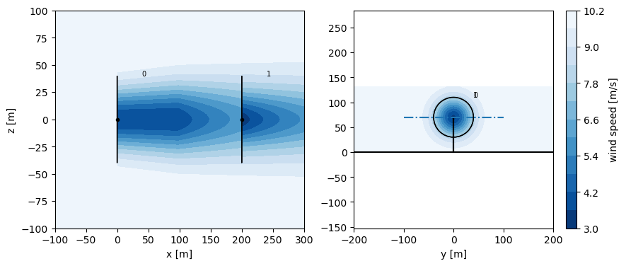
In the plots below, it is clearly seen that the wind speed varies over the rotor, and that the the rotor-average wind speed is not well-defined by the wind sped at the rotor center.

from py_wake.superposition_models import SquaredSum
from py_wake.flow_map import HorizontalGrid, YZGrid
from py_wake import BastankhahGaussian

D = 80
R = D/2
wfm = BastankhahGaussian(site, windTurbines, superpositionModel=SquaredSum())
sim_res = wfm([0,200],[0,0],wd=270,ws=10)

fig,(ax1,ax2) = plt.subplots(1,2, figsize=(10,4))
ax1.set_xlabel("x [m]"), ax1.set_ylabel("y [m]")
sim_res.flow_map(HorizontalGrid(extend=.1)).plot_wake_map(10, ax=ax1, plot_colorbar=False)
sim_res.flow_map(YZGrid(x=199.99)).plot_wake_map(10, ax=ax2)
ax2.plot([-100,100],[70,70],'-.')
ax2.set_xlabel("y [m]"), ax1.set_ylabel("z [m]")

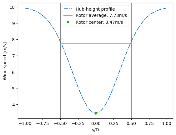
plt.figure()
flow_map = sim_res.flow_map(HorizontalGrid(x=[199.99], y=np.arange(-80, 80)))

for x in [-.5,.5]:
    plt.gca().axvline(x,color='grey')
plt.plot(flow_map.Y[:, 0]/D, flow_map.WS_eff_xylk[:, 0, 0, 0], '-.', label='Hub-height profile')
plt.plot([-.5,.5],[7.73,7.73],label='Rotor average: 7.73m/s')
rc_ws = flow_map.WS_eff_xylk[80, 0, 0, 0]
plt.plot(flow_map.Y[80, 0]/D, rc_ws,'.', ms=10, label='Rotor center: %.2fm/s'%rc_ws)
plt.legend()
plt.xlabel("y/D")
plt.ylabel('Wind speed [m/s]')

/builds/TOPFARM/PyWake/py_wake/deficit_models/gaussian.py:124: UserWarning: The BastankhahGaussian model is not representative of the setup used in the literature. For this, use py_wake.literature.gaussian_models.Bastankhah_PorteAgel_2014 instead
  DeprecatedModel.__init__(self, 'py_wake.literature.gaussian_models.Bastankhah_PorteAgel_2014')

Text(0, 0.5, 'Wind speed [m/s]')

First we create a simple function to model all of the rotor-average models available in PyWake.

from py_wake.rotor_avg_models import RotorCenter, GridRotorAvg, EqGridRotorAvg, GQGridRotorAvg, CGIRotorAvg, PolarGridRotorAvg, PolarRotorAvg, polar_gauss_quadrature, GaussianOverlapAvgModel
from py_wake.flow_map import HorizontalGrid

R=D/2

def plot_rotor_avg_model(rotorAvgModel, name):
    plt.figure()
    m = rotorAvgModel
    wfm = BastankhahGaussian(site,windTurbines,rotorAvgModel=m)
    ws_eff = wfm([0, 200], [0, 0], wd=270, ws=10).WS_eff_ilk[1,0,0]
    plt.title(name)
    c = plt.scatter(m.nodes_x, m.nodes_y,c=m.nodes_weight,label="%.2fm/s"%(ws_eff))
    plt.colorbar(c,label='weight')
    plt.gca().add_artist(plt.Circle((0,0),1,fill=False))
    plt.axis('equal')
    plt.xlabel("y/R"); plt.ylabel('z/R')
    plt.xlim([-1.5,1.5])
    plt.ylim([-1.5,1.5])
    plt.legend()

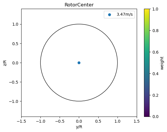
RotorCenter

Setting rotorAvgModel=None determines the rotor average wind speed from the rotor center point. Alternatively, you can use the RotorCenter model which is equivalent.

plot_rotor_avg_model(RotorCenter(), 'RotorCenter')

/builds/TOPFARM/PyWake/py_wake/deficit_models/gaussian.py:124: UserWarning: The BastankhahGaussian model is not representative of the setup used in the literature. For this, use py_wake.literature.gaussian_models.Bastankhah_PorteAgel_2014 instead
  DeprecatedModel.__init__(self, 'py_wake.literature.gaussian_models.Bastankhah_PorteAgel_2014')

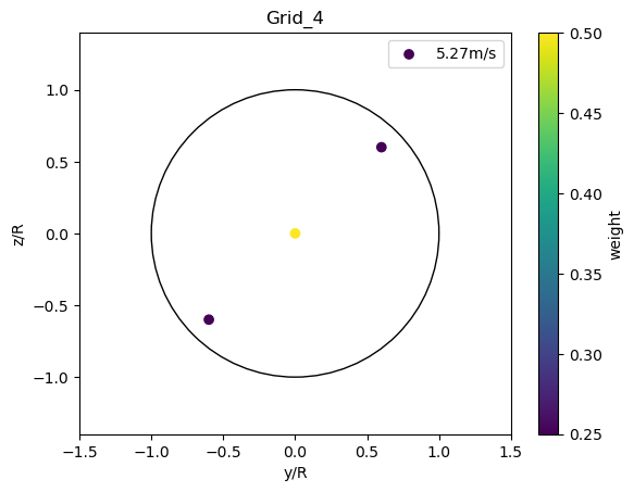
GridRotorAvg

The GridRotorAvg defines a set of points in cartesian coordinates.

x = y = np.array([-.6, 0,.6])
plot_rotor_avg_model(GridRotorAvg(x,y,nodes_weight = [0.25,.5,.25]), 'Grid_4')

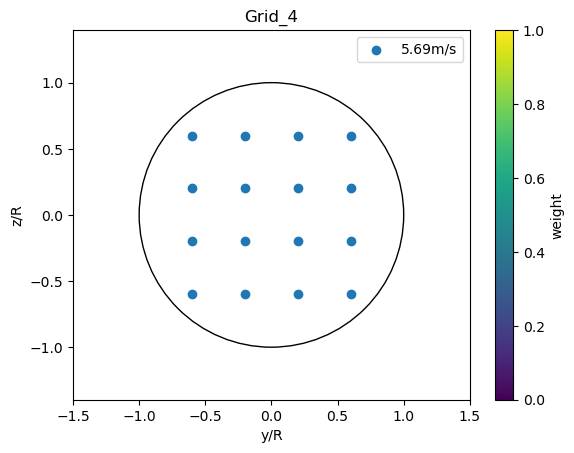
EqGridRotorAvg

The EqGridRotorAvg defines a NxN equidistant cartesian grid of points and discards points outside the rotor.

plot_rotor_avg_model(EqGridRotorAvg(4), 'Grid_4')

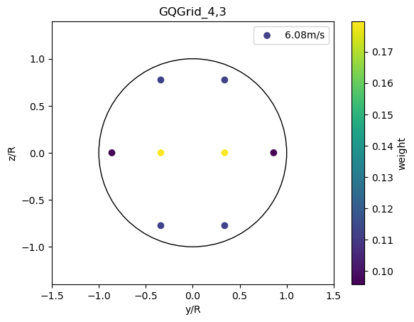
GQGridRotorAvg

The GQGridRotorAvg defines a grid of M x N cartesian grid points using Gaussian quadrature coordinates and weights.

plot_rotor_avg_model(GQGridRotorAvg(4,3), 'GQGrid_4,3')

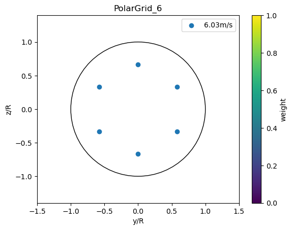
PolarGridRotorAvg

The PolarGridRotorAvg defines a grid in polar coordinates.

theta = np.linspace(-np.pi,np.pi,6, endpoint=False)
r = 2/3
plot_rotor_avg_model(PolarGridRotorAvg(r=r, theta=theta, r_weight=None, theta_weight=None), 'PolarGrid_6')

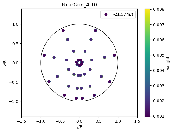
The polar grid can be combined with Gaussian Quadrature.

This is similar to the implementation in FusedWake: https://gitlab.windenergy.dtu.dk/TOPFARM/FUSED-Wake/-/blob/master/fusedwake/gcl/fortran/GCL.f

plot_rotor_avg_model(PolarGridRotorAvg(*polar_gauss_quadrature(4,10)), 'PolarGrid_4,10')

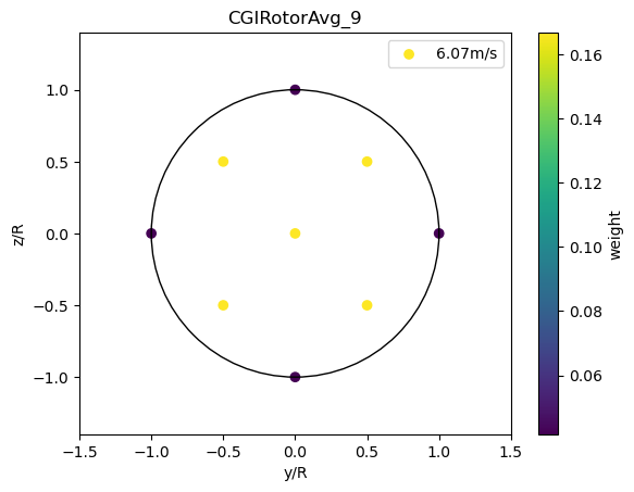
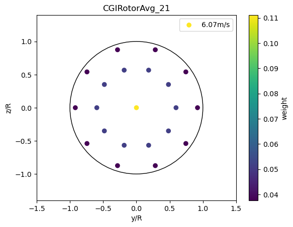
CGIRotorAvg

Circular Gauss integration with 4,7,9 or 21 points as defined in Abramowitz M and Stegun A. Handbook of Mathematical Functions. Dover: New York, 1970.

for n in [4,7,9,21]:
    plot_rotor_avg_model(CGIRotorAvg(n), 'CGIRotorAvg_%d'%n)

AreaOverlapModel

The AreaOverlapModel calculates the fraction of the downstream rotor that is covered by the wake from an upstream wind turbine. This model makes sense for tophat wake deficit models only, e.g. NOJDeficit.

The calculation formula can be found in Eq. (A1) of Feng, J., & Shen, W. Z. (2015). Solving the wind farm layout optimization problem using random search algorithm. Renewable Energy, 78, 182-192. https://doi.org/10.1016/j.renene.2015.01.005

GaussianOverlapAvgModel

The GaussianOverlapModel computes the integral of the gaussian wake deficit over the downstream rotor. To speed up the computation, normalized integrals have been precalculated and stored in a look-up table. This model need the gaussian width parameter, \(\sigma\), and therefore only applies to gaussian wake deficit models. See Appendix A in https://github.com/OrstedRD/TurbOPark/blob/main/TurbOPark%20description.pdf

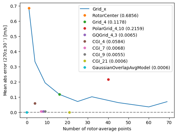
Comparing rotor-average models

In general, the compuational cost and the accuracy of the estimate increases with the number of points, but the distribution of the points also has an impact.

The plot below shows the absolute error of the estimated rotor-average wind speed for the wind directions 270 \(\pm\) 30\(^\circ\) (i.e. wind directions with more than 1% deficit) for a number of different rotor-average models.

grid_models = [EqGridRotorAvg(i) for i in range(1,10)]
wd_lst = np.arange(240,301)

def get_ws_eff(rotorAvgModel):
    wfm = BastankhahGaussian(site,windTurbines,rotorAvgModel=rotorAvgModel)
    return wfm([0, 200], [0, 0], wd=wd_lst, ws=10).WS_eff_ilk[1,:,0]

ws_ref = get_ws_eff(EqGridRotorAvg(200)) # Use 200x200 points (31700 inside the rotor) to determine the reference value

def get_n_err(rotorAvgModel):
    ws_mean_err = np.abs(get_ws_eff(rotorAvgModel) - ws_ref).mean()
    return len(rotorAvgModel.nodes_x), ws_mean_err


plt.gca().axhline(0, color='grey',ls='--')
plt.plot(*zip(*[get_n_err(m) for m in grid_models]), label='Grid_x')
model_lst = [('RotorCenter', EqGridRotorAvg(1)),
             ('Grid_4', EqGridRotorAvg(4)),
             ('PolarGrid_4,10', PolarRotorAvg(*polar_gauss_quadrature(4,10))),
             ('GQGrid_4,3', GQGridRotorAvg(4, 3))] + \
            [('CGI_%d'%n, CGIRotorAvg(n)) for n in [4,7,9,21]]
for name, model in model_lst:
    n,err = get_n_err(model)
    plt.plot(n,err,'.',ms=10, label="%s (%.4f)"%(name,err))
goam_err = np.abs(get_ws_eff(GaussianOverlapAvgModel()) - ws_ref).mean()
plt.plot([0],[goam_err],'.', ms=10, label="GaussianOverlapAvgModel (%.4f)"%(goam_err))
plt.xlabel('Number of rotor-average points')
plt.ylabel(r'Mean abs error (270$\pm30^\circ$) [m/s]')
plt.legend()

<matplotlib.legend.Legend at 0x7f5022d7caf0>