Engineering Wind Farm Models Object

PyWake contains three general engineering wind farm models, namely PropagateDownwind, All2AllIerative and PropagateUpDownIteative.

The table below compares their properties:

/	All2AllIterative	PropagateDownwind	PropagateUpDownIteartive
Includes wakes	Yes	Yes	Yes
Includes blockage	Yes	No	Yes
Memory requirement	High	Low	Low
Simulation speed	Slow	Fast	Medium

In addition different [pre-defined models}(#Predefined-Wind-Farm-Models) exits. The predefined models covers often-used model combinations and models from the literature. I.e. they instantiates one of the above-mentioned wind farm models with a combination of wake deficit models, superposition models, turbulence models, etc. However, these are easily customizable to study the impact of different models on the results.

PropagateDownwind

The PropagateDownwind wind farm model is very fast as it only performs a minimum of deficit calculations. It iterates over all turbines in downstream order. In each iteration it calculates the effective wind speed at the current wind turbine as the free stream wind speed minus the sum of the deficit from upstream sources. Based on this effective wind speed, it calculates the deficit caused by the current turbine on all downstream destinations. Note, that this procedure neglects upstream blockage effects.

for wt in wind turbines in downstream order:
    ws_eff[wt] = ws[wt] - superposition(deficit[from_upstream_src,to_wt])
    ct = windTurbines.ct(ws_eff[wt])
    deficit[from_wt,to_downstream_dst] = wakeDeficitModel(ct, distances[from_wt,to_downstream_dst], ...)

The proceedure is illustrated in the animation below:

• Iteration 1: WT0 sees the free wind (10m/s). Its deficit on WT1 and WT2 is calculated.

• Iteration 2: WT1 sees the free wind minus the deficit from WT0. Its deficit on WT2 is calculated and the effective wind speed at WT2 is updated.

In PyWake, the class is represented as follows:

# Install PyWake if needed
try:
    import py_wake
except ModuleNotFoundError:
    !pip install git+https://gitlab.windenergy.dtu.dk/TOPFARM/PyWake.git

from py_wake.wind_farm_models import PropagateDownwind
help(PropagateDownwind.__init__)

Help on function __init__ in module py_wake.wind_farm_models.engineering_models:

__init__(self, site, windTurbines, wake_deficitModel, superpositionModel=<py_wake.superposition_models.LinearSum object at 0x7f79fa292440>, deflectionModel=None, turbulenceModel=None, rotorAvgModel=None, inputModifierModels=[])
    Initialize flow model

    Parameters
    ----------
    site : Site
        Site object
    windTurbines : WindTurbines
        WindTurbines object representing the wake generating wind turbines
    wake_deficitModel : DeficitModel
        Model describing the wake(downstream) deficit
    rotorAvgModel : RotorAvgModel, optional
        Model defining one or more points at the down stream rotors to
        calculate the rotor average wind speeds from.

        if None, default, the wind speed at the rotor center is used
    superpositionModel : SuperpositionModel
        Model defining how deficits sum up
    deflectionModel : DeflectionModel
        Model describing the deflection of the wake due to yaw misalignment, sheared inflow, etc.
    turbulenceModel : TurbulenceModel
        Model describing the amount of added turbulence in the wake

site and windTurbines and wake_deficitModel are required inputs. By default, the class uses the LinearSum superposition model to add the wakes from upstream turbines.

All2AllIterative

The All2AllIterative wind farm model is slower but is capable of handling blockage effects. It iterates until the effective wind speed converges or it reaches the max number of iterations (number of turbines). The converge tolerance is an input parameter. In each iteration it sums up the deficit from all wind turbine sources and calculates the deficit caused by the all wind turbines turbine on all wind turbines.

while ws_eff not converged:
    ws_eff[all] = ws[all] - superposition(deficit[from_all,to_all])
    ct[all] = windTurbines.ct(ws_eff[all])
    deficit[from_all,to_all] = wakeDeficitModel(ct[all], distances[from_all,to_all], ...)

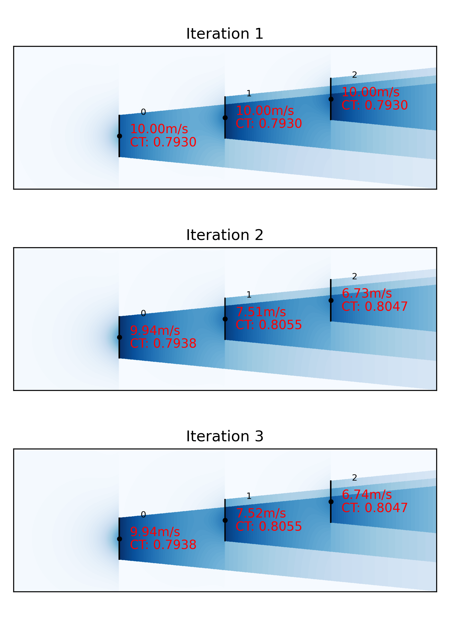
The proceedure is illustrated in the animation below:

• Iteration 1: All three WT see the free wind (10m/s) and their CT values and resulting deficits are therefore equal.

• Iteration 2: The local effective wind speeds are updated taking into account the wake and blockage effects of the other WT. Based on these wind speeds the CT and deficits are recalculated.

• Iteration 3: Repeat after which the flow field has converged.

In PyWake, the class is represented as follows:

from py_wake.wind_farm_models import All2AllIterative
help(All2AllIterative.__init__)

Help on function __init__ in module py_wake.wind_farm_models.engineering_models:

__init__(self, site, windTurbines, wake_deficitModel, superpositionModel=<py_wake.superposition_models.LinearSum object at 0x7f79fa293520>, blockage_deficitModel=None, deflectionModel=None, turbulenceModel=None, convergence_tolerance=1e-06, rotorAvgModel=None, inputModifierModels=[])
    Initialize flow model

    Parameters
    ----------
    site : Site
        Site object
    windTurbines : WindTurbines
        WindTurbines object representing the wake generating wind turbines
    wake_deficitModel : DeficitModel
        Model describing the wake(downstream) deficit
    rotorAvgModel : RotorAvgModel, optional
        Model defining one or more points at the down stream rotors to
        calculate the rotor average wind speeds from.

        if None, default, the wind speed at the rotor center is used
    superpositionModel : SuperpositionModel
        Model defining how deficits sum up
    blockage_deficitModel : DeficitModel
        Model describing the blockage(upstream) deficit
    deflectionModel : DeflectionModel
        Model describing the deflection of the wake due to yaw misalignment, sheared inflow, etc.
    turbulenceModel : TurbulenceModel
        Model describing the amount of added turbulence in the wake
    convergence_tolerance : float or None
        if float: maximum accepted change in WS_eff_ilk [m/s]
        if None: return after first iteration. This only makes sense for benchmark studies where CT,
        wakes and blockage are independent of effective wind speed WS_eff_ilk

In addition to the parameters specified in the PropagateDownwind class, here we determine a convergence tolerance in terms of the maximum accepted change in WS_eff_ilk in m/s. In this case, the blockage deficit model is set to None as default, but this should be changed depending on the engineering wind farm model used.

As default, the All2AllIterative simulation runs a PropagateDownwind simulation during initialization and uses the resulting effective wind speed as starting condition for its own iterative process.

PropagateUpDownIterative

The PropagateUpDownIterative wind farm model combines the approaches of PropagateDownwind and All2AllIterative

• Iteration 1 (Propagate wake down):

  • Iteration 1.1: WT0 sees the free wind (10m/s). Its wake deficit on WT1 and WT2 is calculated.

  • Iteration 1.2: WT1 sees the free wind minus the wake deficit from WT0. Its wake deficit on WT2 is calculated and the effective wind speed at WT2 is updated.

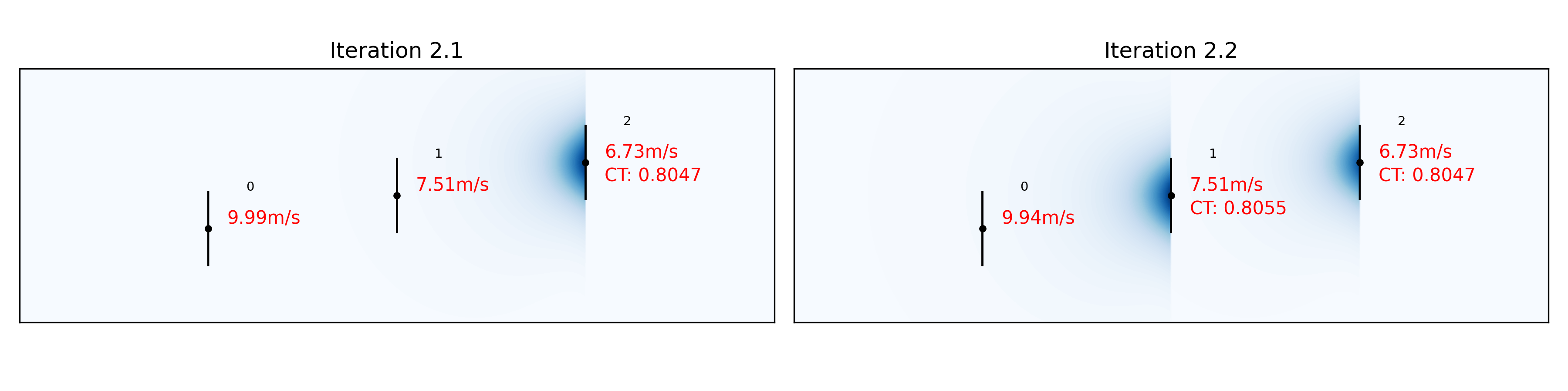
• Iteration 2 (Propagate blockage up)

  • Iteration 2.1: All wind turbines see the free wind speed minus the wake deficit obtained in iteration 1. WT2 sees 6.73m/s and its blockage deficit on WT1 and WT0 is calculated.

  • Iteration 2.2: WT1 sees the free wind speed minus the wake deficit obtained in iteration 1 and the blockage deficit from WT2. Its blockage deficit on WT0 is calculated and the effective wind speed at WT0 is updated.

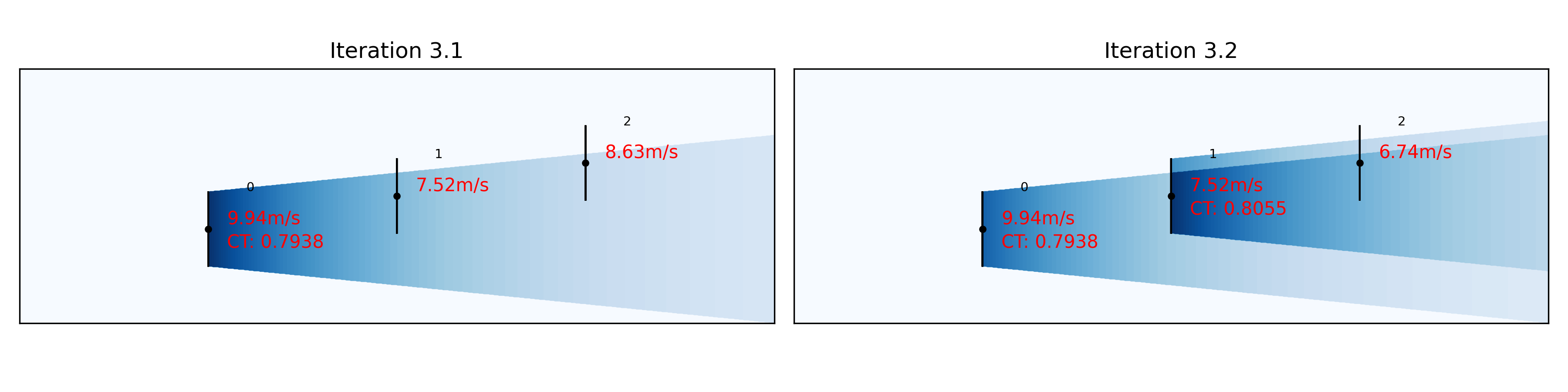
• Iteration 3 (Propagate wake down):

  • Iteration 3.1: All wind turbines see the free wind minus the blockage obtained in iteration 2. WT0 seees 9.94 m/s and its wake deficit on WT1 and WT2 is calculated.

  • Iteration 3.2: WT1 sees the free wind minus the blockage deficit obtained in iteration 2 and the wake deficit from WT0. Its wake deficit on WT2 is calculated and the effective wind speed at WT2 is updated.

• Iteration 4 (Propagate blockage up)

  • Iteration 4.1: All wind turbines see the free wind speed minus the wake deficit obtained in iteration 3. WT2 sees 6.74m/s and its blockage deficit on WT1 and WT0 is calculated.

  • Iteration 4.2: WT1 sees the free wind speed minus the wake deficit obtained in iteration 3 and the blockage deficit from WT2. Its blockage deficit on WT0 is calculated and the effective wind speed at WT0 is updated.

The constructor of PropagateUpDownIterative is very similar to the constructor of All2AllIterative:

from py_wake.wind_farm_models import PropagateUpDownIterative
help(PropagateUpDownIterative.__init__)

Help on function __init__ in module py_wake.wind_farm_models.engineering_models:

__init__(self, site, windTurbines, wake_deficitModel, superpositionModel=<py_wake.superposition_models.LinearSum object at 0x7f79fa2923e0>, blockage_deficitModel=None, deflectionModel=None, turbulenceModel=None, rotorAvgModel=None, inputModifierModels=[], convergence_tolerance=1e-06)
    Initialize flow model

    Parameters
    ----------
    site : Site
        Site object
    windTurbines : WindTurbines
        WindTurbines object representing the wake generating wind turbines
    wake_deficitModel : DeficitModel
        Model describing the wake(downstream) deficit
    rotorAvgModel : RotorAvgModel, optional
        Model defining one or more points at the down stream rotors to
        calculate the rotor average wind speeds from.

        if None, default, the wind speed at the rotor center is used
    superpositionModel : SuperpositionModel
        Model defining how deficits sum up
    deflectionModel : DeflectionModel
        Model describing the deflection of the wake due to yaw misalignment, sheared inflow, etc.
    turbulenceModel : TurbulenceModel
        Model describing the amount of added turbulence in the wake

Predefined Wind Farm Models

The pre-defines wind farm models are adapted from the literature, where their corresponding default superposition model, turbulence model and calibration parameters are taken from the paper describing each model.

The engineering wind farm models comprise:

Reference	Name	WindFarm Model	Wake Deficit Model	Blockage Deficit Model	Superposition Model	Turbulence Model
1	Jensen_1983	PropagateDownwind	NOJDeficit		SquaredSum
2	Ott_Nielsen_2014	PropagateDownwind	FugaDeficit		LinearSum
3	Ott_Nielsen_2014_Blockage	All2AllIterative	FugaDeficit	FugaDeficit	LinearSum
4	Bastankhah_PorteAgel_2014	PropagateDownwind	BastankhahGa ussianDeficit		SquaredSum
5	IEA37CaseStudy1	PropagateDownwind	IEA37SimpleBastankhahGaussianDefic it		SquaredSum
6	Niayifar_PorteAgel_2016	PropagateDownwind	Niayifar GaussianDeficit		LinearSum	CrespoHernandez
7	Zong_PorteAgel_2020	PropagateDownwind	` ZongGaussianDeficit <WakeDeficitModels.ipynb#ZongGaussianDeficit>`__		WeightedSum	CrespoHernandez
8	Nygaard_2022	PropagateDownwind	Tu rboGaussianDeficit		SquaredSum
9	Blondel_Cathelain_2020	PropagateDownwind	BlondelSuperG aussianDeficit2020		LinearSum

• Default rotor-average model: RotorCenter

• Default turbulence model: None

All models require a Site and a WindTurbine object to run, and each of them may require additional inputs such as calibration parameters. The parameters shown are the default and used in the literature, but if necessary, they can be modified to better suit a particular case study.

In the case of Fuga, a file with look up tables is needed; the file is created by specifying the turbine’s rotor diameter, hub height and roughness length of the site to study.

For information on the calculation of the velocity deficit for each model, please refer to the Wake Deficit Models notebook.

Below are some examples of different wind farm models under the PropagateDownwind base class. The full set of pre-defined wind farm models can be found in PyWake’s repository under the literature folder.

1) Bastankhah Gaussian

class Bastankhah_PorteAgel_2014(PropagateDownwind):
def __init__(self, site, windTurbines, k=0.0324555, ceps=.2, ct2a=ct2a_madsen, use_effective_ws=False,
                 rotorAvgModel=None, superpositionModel=SquaredSum(),
                 deflectionModel=None, turbulenceModel=None, groundModel=None):

2) Niayifar Gaussian

class Niayifar_PorteAgel_2016(PropagateDownwind):
def __init__(self, site, windTurbines, a=[0.38, 4e-3], ceps=.2, superpositionModel=LinearSum(),
                 deflectionModel=None, turbulenceModel=CrespoHernandez(), rotorAvgModel=None, groundModel=None,
                 use_effective_ws=True, use_effective_ti=True):

3) Zong Gaussian

class Zong_PorteAgel_2020(PropagateDownwind):
def __init__(self, site, windTurbines, a=[0.38, 4e-3], deltawD=1. / np.sqrt(2), lam=7.5, B=3,
                 rotorAvgModel=None, superpositionModel=WeightedSum(), deflectionModel=None,
                 turbulenceModel=CrespoHernandez(), groundModel=None, use_effective_ws=True, use_effective_ti=True):

3) TurbOPark

class Nygaard_2022(PropagateDownwind):
def __init__(self, site, windTurbines):

        wake_deficitModel = TurboGaussianDeficit(
            ct2a=ct2a_mom1d,
            groundModel=Mirror(),
            rotorAvgModel=GaussianOverlapAvgModel())

4) Fuga

class Ott_Nielsen_2014(PropagateDownwind):
    def __init__(self, LUT_path, site, windTurbines,
                 rotorAvgModel=None, deflectionModel=None, turbulenceModel=None, remove_wriggles=False):

In addition, Fuga’s wind farm model comes with the possibility of modeling blockage. For this, the All2AllIterative base class is used.

class Ott_Nielsen_2014_Blockage(All2AllIterative):
    def __init__(self, LUT_path, site, windTurbines, rotorAvgModel=None,
                 deflectionModel=None, turbulenceModel=None, convergence_tolerance=1e-6, remove_wriggles=False):