Experiment: Combine Models

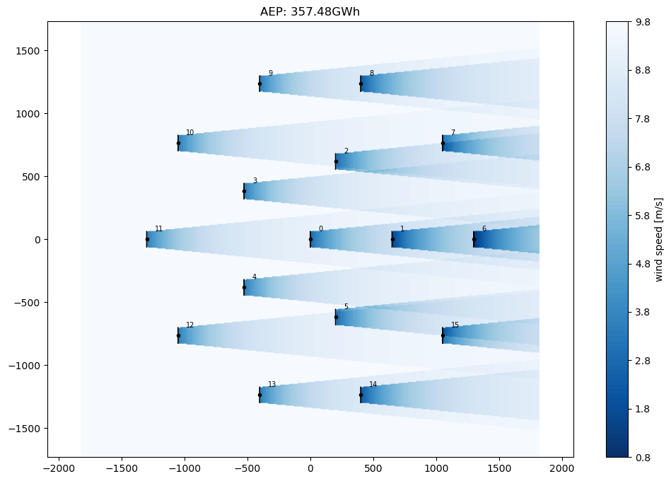
In this notebook, you can combine the difference models of PyWake and see the effects in terms of AEP and a flow map.

Install PyWake if needed

# Install PyWake if needed
try:
    import py_wake
except ModuleNotFoundError:
    !pip install git+https://gitlab.windenergy.dtu.dk/TOPFARM/PyWake.git

Now we also import all available models

from py_wake.deficit_models import *
from py_wake.deficit_models.deficit_model import *
from py_wake.wind_farm_models import *
from py_wake.rotor_avg_models import *
from py_wake.superposition_models import *
from py_wake.deflection_models import *
from py_wake.turbulence_models import *
from py_wake.ground_models import *
from py_wake.deficit_models.utils import *

Then, we set up the site, wind turbines as well as their initial positions.

from py_wake.examples.data.iea37._iea37 import IEA37Site, IEA37_WindTurbines

site = IEA37Site(16)
windTurbines = IEA37_WindTurbines()
x,y = site.initial_position.T

# prepare for the model combination tool
from py_wake.utils.model_utils import get_models, get_signature
from ipywidgets import interact
from IPython.display import HTML, display, Javascript
import time
import matplotlib.pyplot as plt

# Fix ipywidget label width
display(HTML('''<style>.widget-label { min-width: 20ex !important; }</style>'''))

def print_signature(windFarmModel, **kwargs):
    s = """# windFarmModel autogenerated by dropdown boxes
t = time.time()
wfm = %s
sim_res = wfm(x,y)
plt.figure(figsize=(12,8))
sim_res.flow_map(wd=270).plot_wake_map()
print (wfm)
print ("Computation time (AEP + flowmap):", time.time()-t)
plt.title('AEP: %%.2fGWh'%%(sim_res.aep().sum()))"""% get_signature(windFarmModel, kwargs, 1)
    # Write windFarmModel code to cell starting "# windFarmModel autogenerated by dropdown boxes"
    display(Javascript("""
for (var cell of IPython.notebook.get_cells()) {
    if (cell.get_text().startsWith("# windFarmModel autogenerated by dropdown boxes")){
        cell.set_text(`%s`);
        cell.execute();
    }
}"""%s))

# setup list of models
models = {n:[(getattr(m,'__name__',m), m) for m in get_models(cls)]
          for n,cls in [('windFarmModel', WindFarmModel),
                        ('wake_deficitModel', WakeDeficitModel),
                        ('rotorAvgModel', RotorAvgModel),
                        ('superpositionModel', SuperpositionModel),
                        ('blockage_deficitModel', BlockageDeficitModel),
                        ('deflectionModel',DeflectionModel),
                        ('turbulenceModel', TurbulenceModel),
                        ('groundModel', GroundModel)
                        ]}

Combine and execute model

Combine your model via the dropdown boxes below.

Choosing a different model updates and executes the the code cell below which runs the wind farm model, prints the AEP and plots a flow map.

_ = interact(print_signature, **models)

# windFarmModel autogenerated by dropdown boxes
t = time.time()
wfm = PropagateDownwind(
    site,
    windTurbines,
    wake_deficitModel=NOJDeficit(
        k=0.1,
        rotorAvgModel=AreaOverlapAvgModel(),
        groundModel=None),
    superpositionModel=LinearSum(),
    deflectionModel=None,
    turbulenceModel=None,
    rotorAvgModel=None)
sim_res = wfm(x,y)
plt.figure(figsize=(12,8))
sim_res.flow_map(wd=270).plot_wake_map()
print (wfm)
print ("Computation time (AEP + flowmap):", time.time()-t)
plt.title('AEP: %.2fGWh'%(sim_res.aep().sum()))

PropagateDownwind(PropagateUpDownIterative, NOJDeficit-wake, LinearSum-superposition)
Computation time (AEP + flowmap): 0.6689565181732178

Text(0.5, 1.0, 'AEP: 357.48GWh')