Quickstart

In this tutorial, the basic capabilities of PyWake are shown. Essentially, how to calculate a wind farm’s AEP using the wind farm simulation tool and how to visualize and interpret the results. In addition, the use of flow maps is also shown.

Install PyWake if needed

# Install PyWake if needed
try:
    import py_wake
except ModuleNotFoundError:
    !pip install git+https://gitlab.windenergy.dtu.dk/TOPFARM/PyWake.git

Import and set up of wind turbines, site, and flow model

There are many sites and wind turbines available in PyWake, some of them include:

• Hornsrev1 offshore wind farm

• Lillgrund offshore wind farm

• IEA Task 37 Site land-based wind farm

• Vestas V80 turbine

• IEA 3.4 MW turbine

• DTU 10MW reference turbine

For detailed information on the sites and wind turbine object features, please see the Site and Wind turbine examples.

from py_wake.examples.data.hornsrev1 import Hornsrev1Site, V80, wt_x, wt_y, wt16_x, wt16_y
from py_wake import NOJ

#here we import the turbine, site and wake deficit model to use.
windTurbines = V80()
site = Hornsrev1Site()
noj = NOJ(site,windTurbines)

/builds/TOPFARM/PyWake/py_wake/deficit_models/noj.py:84: UserWarning: The NOJ model is not representative of the setup used in the literature. For this, use py_wake.literature.noj.Jensen_1983 instead
  DeprecatedModel.__init__(self, 'py_wake.literature.noj.Jensen_1983')

Now we run the model using the initial positions of the wind farm

For more information about the SimulationResult object and the paratemers included, please see the wind farm simulation example.

simulationResult = noj(wt16_x,wt16_y)

To calculate the AEP, we use the simulationResult.aep() command. This will show an xarray with the characteristics of the site, including the number of turbines and the wind speed and wind direction studied. In addition, it will show the AEP of each turbine for each flow case.

simulationResult.aep()

<xarray.DataArray 'AEP [GWh]' (wt: 16, wd: 360, ws: 23)> Size: 1MB
array([[[0.00000000e+00, 4.99347385e-05, 1.42930180e-04, ...,
         2.47780973e-06, 1.00529802e-06, 3.84203469e-07],
        [0.00000000e+00, 4.99347385e-05, 1.42930180e-04, ...,
         2.47780973e-06, 1.00529802e-06, 3.84203469e-07],
        [0.00000000e+00, 4.99347385e-05, 1.42930180e-04, ...,
         2.47780973e-06, 1.00529802e-06, 3.84203469e-07],
        ...,
        [0.00000000e+00, 4.99347385e-05, 1.42930180e-04, ...,
         2.47780973e-06, 1.00529802e-06, 3.84203469e-07],
        [0.00000000e+00, 4.99347385e-05, 1.42930180e-04, ...,
         2.47780973e-06, 1.00529802e-06, 3.84203469e-07],
        [0.00000000e+00, 4.99347385e-05, 1.42930180e-04, ...,
         2.47780973e-06, 1.00529802e-06, 3.84203469e-07]],

       [[0.00000000e+00, 3.21704038e-05, 1.07631358e-04, ...,
         2.47780973e-06, 1.00529802e-06, 3.84203469e-07],
        [0.00000000e+00, 3.50325965e-05, 1.13318710e-04, ...,
         2.47780973e-06, 1.00529802e-06, 3.84203469e-07],
        [0.00000000e+00, 3.81343279e-05, 1.19482041e-04, ...,
         2.47780973e-06, 1.00529802e-06, 3.84203469e-07],
...
        [0.00000000e+00, 3.70751758e-05, 9.95804636e-05, ...,
         2.47780973e-06, 1.00529802e-06, 3.84203469e-07],
        [0.00000000e+00, 3.70626513e-05, 9.95068465e-05, ...,
         2.47780973e-06, 1.00529802e-06, 3.84203469e-07],
        [0.00000000e+00, 3.73276423e-05, 1.00421384e-04, ...,
         2.47780973e-06, 1.00529802e-06, 3.84203469e-07]],

       [[0.00000000e+00, 3.69047609e-05, 1.05287023e-04, ...,
         2.47780973e-06, 1.00529802e-06, 3.84203469e-07],
        [0.00000000e+00, 3.86957286e-05, 1.12417512e-04, ...,
         2.47780973e-06, 1.00529802e-06, 3.84203469e-07],
        [0.00000000e+00, 4.06849605e-05, 1.19260253e-04, ...,
         2.47780973e-06, 1.00529802e-06, 3.84203469e-07],
        ...,
        [0.00000000e+00, 3.54284013e-05, 9.86539322e-05, ...,
         2.47780973e-06, 1.00529802e-06, 3.84203469e-07],
        [0.00000000e+00, 3.54109110e-05, 9.85789848e-05, ...,
         2.47780973e-06, 1.00529802e-06, 3.84203469e-07],
        [0.00000000e+00, 3.55351507e-05, 9.93005262e-05, ...,
         2.47780973e-06, 1.00529802e-06, 3.84203469e-07]]])
Coordinates:
  * ws       (ws) int64 184B 3 4 5 6 7 8 9 10 11 ... 17 18 19 20 21 22 23 24 25
  * wd       (wd) int64 3kB 0 1 2 3 4 5 6 7 ... 352 353 354 355 356 357 358 359
  * wt       (wt) int64 128B 0 1 2 3 4 5 6 7 8 9 10 11 12 13 14 15
    type     (wt) int64 128B 0 0 0 0 0 0 0 0 0 0 0 0 0 0 0 0
Attributes:
    Description:  Annual energy production [GWh]

xarray.DataArray

'AEP [GWh]'

• wt: 16
• wd: 360
• ws: 23

• 0.0 4.993e-05 0.0001429 0.0002968 ... 2.478e-06 1.005e-06 3.842e-07

  array([[[0.00000000e+00, 4.99347385e-05, 1.42930180e-04, ...,
           2.47780973e-06, 1.00529802e-06, 3.84203469e-07],
          [0.00000000e+00, 4.99347385e-05, 1.42930180e-04, ...,
           2.47780973e-06, 1.00529802e-06, 3.84203469e-07],
          [0.00000000e+00, 4.99347385e-05, 1.42930180e-04, ...,
           2.47780973e-06, 1.00529802e-06, 3.84203469e-07],
          ...,
          [0.00000000e+00, 4.99347385e-05, 1.42930180e-04, ...,
           2.47780973e-06, 1.00529802e-06, 3.84203469e-07],
          [0.00000000e+00, 4.99347385e-05, 1.42930180e-04, ...,
           2.47780973e-06, 1.00529802e-06, 3.84203469e-07],
          [0.00000000e+00, 4.99347385e-05, 1.42930180e-04, ...,
           2.47780973e-06, 1.00529802e-06, 3.84203469e-07]],
  
         [[0.00000000e+00, 3.21704038e-05, 1.07631358e-04, ...,
           2.47780973e-06, 1.00529802e-06, 3.84203469e-07],
          [0.00000000e+00, 3.50325965e-05, 1.13318710e-04, ...,
           2.47780973e-06, 1.00529802e-06, 3.84203469e-07],
          [0.00000000e+00, 3.81343279e-05, 1.19482041e-04, ...,
           2.47780973e-06, 1.00529802e-06, 3.84203469e-07],
  ...
          [0.00000000e+00, 3.70751758e-05, 9.95804636e-05, ...,
           2.47780973e-06, 1.00529802e-06, 3.84203469e-07],
          [0.00000000e+00, 3.70626513e-05, 9.95068465e-05, ...,
           2.47780973e-06, 1.00529802e-06, 3.84203469e-07],
          [0.00000000e+00, 3.73276423e-05, 1.00421384e-04, ...,
           2.47780973e-06, 1.00529802e-06, 3.84203469e-07]],
  
         [[0.00000000e+00, 3.69047609e-05, 1.05287023e-04, ...,
           2.47780973e-06, 1.00529802e-06, 3.84203469e-07],
          [0.00000000e+00, 3.86957286e-05, 1.12417512e-04, ...,
           2.47780973e-06, 1.00529802e-06, 3.84203469e-07],
          [0.00000000e+00, 4.06849605e-05, 1.19260253e-04, ...,
           2.47780973e-06, 1.00529802e-06, 3.84203469e-07],
          ...,
          [0.00000000e+00, 3.54284013e-05, 9.86539322e-05, ...,
           2.47780973e-06, 1.00529802e-06, 3.84203469e-07],
          [0.00000000e+00, 3.54109110e-05, 9.85789848e-05, ...,
           2.47780973e-06, 1.00529802e-06, 3.84203469e-07],
          [0.00000000e+00, 3.55351507e-05, 9.93005262e-05, ...,
           2.47780973e-06, 1.00529802e-06, 3.84203469e-07]]])

• Coordinates: (4)
  • ws
    (ws)
    int64
    3 4 5 6 7 8 9 ... 20 21 22 23 24 25

    Description :

    Ambient reference wind speed [m/s]

    array([ 3,  4,  5,  6,  7,  8,  9, 10, 11, 12, 13, 14, 15, 16, 17, 18, 19, 20,
           21, 22, 23, 24, 25])

  • wd
    (wd)
    int64
    0 1 2 3 4 5 ... 355 356 357 358 359

    Description :

    Ambient reference wind direction [deg]

    array([  0,   1,   2, ..., 357, 358, 359])

  • wt
    (wt)
    int64
    0 1 2 3 4 5 6 ... 10 11 12 13 14 15

    Description :

    Wind turbine number

    array([ 0,  1,  2,  3,  4,  5,  6,  7,  8,  9, 10, 11, 12, 13, 14, 15])

  • type
    (wt)
    int64
    0 0 0 0 0 0 0 0 0 0 0 0 0 0 0 0

    Description :

    Wind turbine type

    array([0, 0, 0, 0, 0, 0, 0, 0, 0, 0, 0, 0, 0, 0, 0, 0])

• Indexes: (3)
  • ws
    PandasIndex

    PandasIndex(Index([ 3,  4,  5,  6,  7,  8,  9, 10, 11, 12, 13, 14, 15, 16, 17, 18, 19, 20,
           21, 22, 23, 24, 25],
          dtype='int64', name='ws'))

  • wd
    PandasIndex

    PandasIndex(Index([  0,   1,   2,   3,   4,   5,   6,   7,   8,   9,
           ...
           350, 351, 352, 353, 354, 355, 356, 357, 358, 359],
          dtype='int64', name='wd', length=360))

  • wt
    PandasIndex

    PandasIndex(Index([0, 1, 2, 3, 4, 5, 6, 7, 8, 9, 10, 11, 12, 13, 14, 15], dtype='int64', name='wt'))

• Attributes: (1)

  Description :

  Annual energy production [GWh]

To obtain the total AEP, we use the .sum() command.

print ("Total AEP: %f GWh"%simulationResult.aep().sum())

Total AEP: 143.074909 GWh

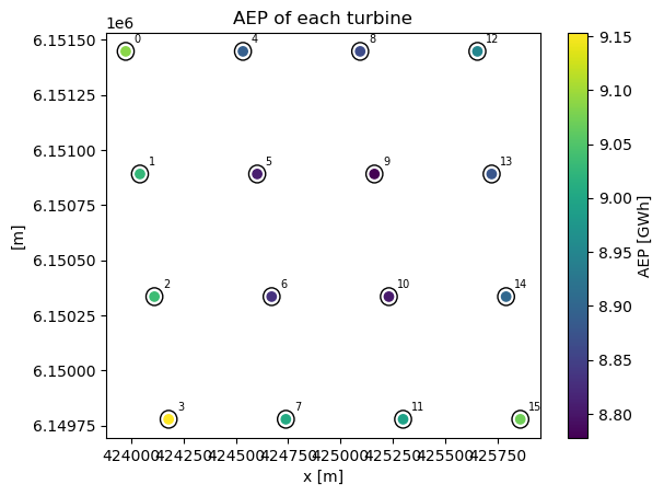
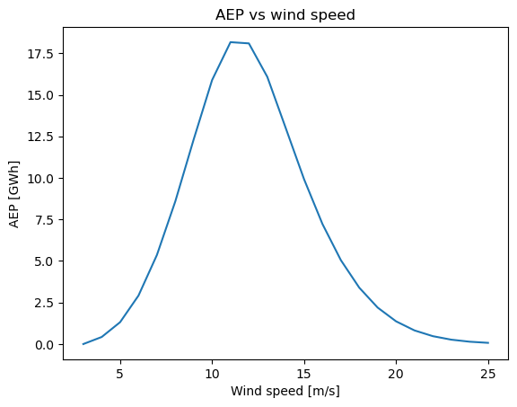
Plot AEP as function of wind turbines, wind direction and wind speed

There is also the possibility of plotting the individual AEP for each turbine for the flow cases studied. In addition, the AEP can be plotted against either the wind speed or wind direction.

import matplotlib.pyplot as plt
%matplotlib inline

plt.figure()
aep = simulationResult.aep()
windTurbines.plot(wt16_x,wt16_y)
c =plt.scatter(wt16_x, wt16_y, c=aep.sum(['wd','ws']))
plt.colorbar(c, label='AEP [GWh]')
plt.title('AEP of each turbine')
plt.xlabel('x [m]')
plt.ylabel('[m]')

plt.figure()
aep.sum(['wt','wd']).plot()
plt.xlabel("Wind speed [m/s]")
plt.ylabel("AEP [GWh]")
plt.title('AEP vs wind speed')

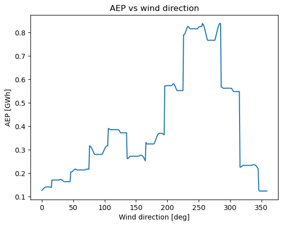
plt.figure()
aep.sum(['wt','ws']).plot()
plt.xlabel("Wind direction [deg]")
plt.ylabel("AEP [GWh]")
plt.title('AEP vs wind direction')

Text(0.5, 1.0, 'AEP vs wind direction')

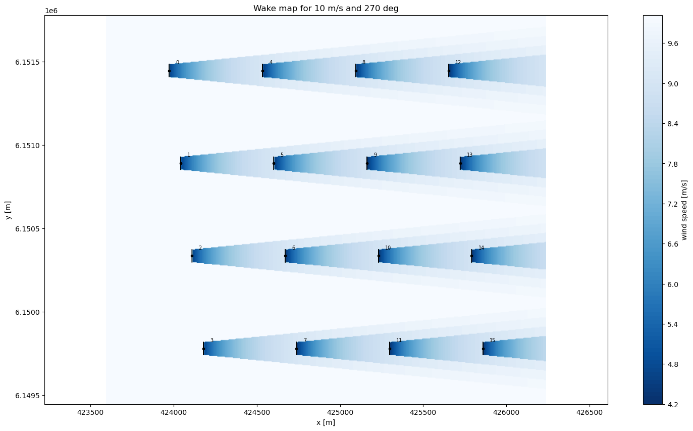
Plot flow maps

It is also possible to plot the wind farm wake map. This shows the wake behavior for each turbine given the flow cases studied.

You can change the values of the wind speed and wind direction to visualize the wake maps for different flow cases.

wind_speed = 10
wind_direction = 270

plt.figure()
flow_map = simulationResult.flow_map(ws=wind_speed, wd=wind_direction)
plt.figure(figsize=(18,10))
flow_map.plot_wake_map()
plt.xlabel('x [m]')
plt.ylabel('y [m]')
plt.title('Wake map for' + f' {wind_speed} m/s and {wind_direction} deg')

Text(0.5, 1.0, 'Wake map for 10 m/s and 270 deg')