Experiment: Improve Hornsrev1 Layout

In this exercise, you can investigate how changing the turbine positions inside the Hornsrev1 wind farm influences its AEP.

Install PyWake if needed

# Install PyWake if needed
try:
    import py_wake
except ModuleNotFoundError:
    !pip install git+https://gitlab.windenergy.dtu.dk/TOPFARM/PyWake.git

First we import basic Python elements

import numpy as np
import matplotlib.pyplot as plt

Import and instantiate relevant PyWake objects

We operate with four fundamental objects in PyWake, namely Site, WindTurbines and WindFarmModel, as explained in the Overview section.

#importing the properties of Hornsrev1, which are already stored in PyWake
from py_wake.examples.data.hornsrev1 import V80
from py_wake.examples.data.hornsrev1 import Hornsrev1Site
from py_wake.examples.data.hornsrev1 import wt_x, wt_y

# BastankhahGaussian combines the engineering wind farm model, `PropagateDownwind` with
# the `BastankhahGaussianDeficit` wake deficit model and the `SquaredSum` super position model
from py_wake.literature.gaussian_models import Bastankhah_PorteAgel_2014

# After we import the objects we instatiate them:
site = Hornsrev1Site()
wt = V80()
windFarmModel = Bastankhah_PorteAgel_2014(site, wt, k=0.0324555)

The Site object

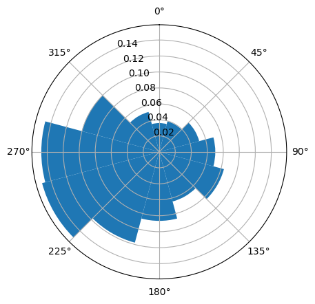
There are multiple functionalities available from the Site object as well as wind conditions, probability and geometry of the wind farm. We can e.g. plot the wind rose with a specific number of bins by using the plot_wd_distribution function:

site.plot_wd_distribution(n_wd=12);

The WindTurbine object

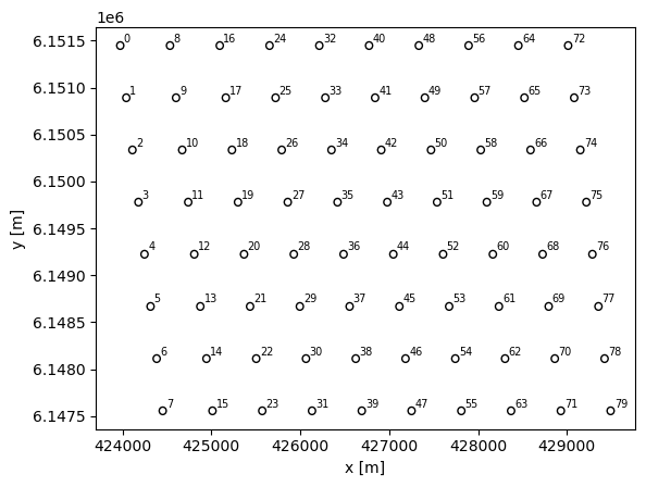
The Wind turbine object contains relevant information about the turbine used as well as supplying usefull functions. It holds information about the power curve, ct-curve, hub height and diameter and has a plotting function to visualize the layout of the turbines.

# Original layout
plt.figure()
wt.plot(wt_x, wt_y)
plt.xlabel('x [m]')
plt.ylabel('y [m]')

Text(0, 0.5, 'y [m]')

AEP Calculation

# Original AEP
aep_ref = windFarmModel(wt_x,wt_y).aep().sum()
print ('Original AEP: %f GWh'%aep_ref)

Original AEP: 664.334531 GWh

Exercise: Improve the AEP by modifying turbine locations.

Modify the x and y offsets for the rows and columns to increase the AEP.

Note, the turbines positions are limited by a rectangle surrounding the existing layout.

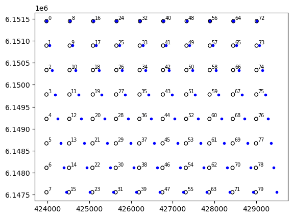
# Here we define a function to print and plot your new layout. No need to change anything here
def add_offset_plot_and_print(row_offset_x, row_offset_y, col_offset_x, col_offset_y):
    x,y = wt_x, wt_y
    y = np.reshape(y,(10,8)).astype(float)
    x = np.reshape(x,(10,8)).astype(float)

    x+= np.array(row_offset_x)
    y+= np.array(row_offset_y)
    x+= np.array(col_offset_x)[:,np.newaxis]
    y+= np.array(col_offset_y)[:,np.newaxis]
    y = np.maximum(min(wt_y), np.minimum(max(wt_y), y.flatten()))
    x = np.maximum(min(wt_x), np.minimum(max(wt_x), x.flatten()))

    plt.plot()
    plt.plot(wt_x, wt_y,'b.')
    wt.plot(x, y)
    aep = windFarmModel(x,y).aep().sum()
    print ("AEP ref", aep_ref.values)
    print ("AEP", aep.values)
    print ("Increase: %f %%"%((aep-aep_ref)/aep_ref*100))

Now try to modify the row and column offsets and see if you can improve the AEP

# =======================================
# Specify offsets
# =======================================

row_offset_x = np.linspace(0,1,8)* -500
row_offset_y = np.linspace(0,1,8) * 0

col_offset_x = np.linspace(0,1,10) * 0
col_offset_y = np.linspace(0,1,10) * 0

add_offset_plot_and_print(row_offset_x, row_offset_y, col_offset_x, col_offset_y)

AEP ref 664.3345305655693
AEP 664.4739841319365
Increase: 0.020991 %