![]()
Roads and Cables
Try this yourself (requires google account)
In this example, a layout optimization with the Internal Rate of Return (IRR) as the objective function is performed. The cost of cables and electrical grid cable components are specified within the cost model to see how these are incorporated into the optimization and their influence on the results. Both the NREL and DTU cost model can be selected to perform the optimizations and analyze their differences.
Install TOPFARM if needed
[ ]:
# Install TopFarm if needed
import importlib
if not importlib.util.find_spec("topfarm"):
    !pip install git+https://gitlab.windenergy.dtu.dk/TOPFARM/TopFarm2.git
In colab, use the “inline” backend
[1]:
# non-updating, inline plots
%matplotlib inline
import warnings
warnings.filterwarnings('ignore')
# ...or updating plots in new window
#%matplotlib qt
First, let’s import a few TOPFARM classes and basic Python elements
In addition the the common TOPFARM elements such as the CostModelComponent, TopFarmProblem, optimization driver and constraints, here we are importing some electrical components that will calculate the influence of cabling costs in the optimization.
ElNetCost will calculate the cost associated to the electrical connection in the wind farm, considering the cost per meter cable used. This cost will serve as input to the IRR calculation alongside the AEP of the wind farm, to obtain the total IRR when cabling is added to the optimization problem.
[2]:
import numpy as np
import matplotlib.pylab as plt

from topfarm.cost_models.cost_model_wrappers import CostModelComponent
from topfarm import TopFarmGroup, TopFarmProblem
from topfarm.easy_drivers import EasyRandomSearchDriver, EasyScipyOptimizeDriver
from topfarm.drivers.random_search_driver import RandomizeTurbinePosition_Circle
from topfarm.constraint_components.spacing import SpacingConstraint
from topfarm.constraint_components.boundary import XYBoundaryConstraint
from topfarm.cost_models.electrical.simple_msp import ElNetLength, ElNetCost, XYCablePlotComp
from topfarm.cost_models.utils.spanning_tree import mst

#classes to define the site to use
from py_wake.site import UniformWeibullSite
from py_wake.site.shear import PowerShear
We create a function to set up the site wind speed conditions and the turbines’ initial positions. Since the UniformWeibullSite will be used, which describes a site with uniform and Weibull distributed wind speed. Some key parameters must be specified:
the probability of wind direction sector, f
the Weibull shape parameter, k
the Weibull scale parameter, A
In addition, the turbulence intensity and shear exponent are selected.
[3]:
def get_site():
    f = [0.035972, 0.039487, 0.051674, 0.070002, 0.083645, 0.064348,
            0.086432, 0.117705, 0.151576, 0.147379, 0.10012, 0.05166]
    A = [9.176929, 9.782334, 9.531809, 9.909545, 10.04269, 9.593921,
        9.584007, 10.51499, 11.39895, 11.68746, 11.63732, 10.08803]
    k = [2.392578, 2.447266, 2.412109, 2.591797, 2.755859, 2.595703,
        2.583984, 2.548828, 2.470703, 2.607422, 2.626953, 2.326172]
    ti = 0.001
    h_ref = 100
    alpha = .1

    site = UniformWeibullSite(f, A, k, ti, shear=PowerShear(h_ref=h_ref, alpha=alpha))

    #setting up the initial turbine positions
    spacing = 2000
    N = 5  #number of turbines per row
    theta = 76  #inclination angle of turbines
    dx = np.tan(np.radians(theta))
    x = np.array([np.linspace(0,(N-1)*spacing,N)+i*spacing/dx for i in range(N)])
    y = np.array(np.array([N*[i*spacing] for i in range(N)]))
    initial_positions = np.column_stack((x.ravel(),y.ravel()))
    eps = 2000
    delta = 5
    site.boundary = np.array([(0-delta, 0-delta),
                        ((N-1)*spacing+eps, 0-delta),
                        ((N-1)*spacing*(1+1/dx)+eps*(1+np.cos(np.radians(theta))), (N-1)*spacing+eps*np.sin(np.radians(theta))-delta),
                        ((N-1)*spacing/dx+eps*np.cos(np.radians(theta)), (N-1)*spacing+eps*np.sin(np.radians(theta)))])
    site.initial_position = initial_positions
    return site
Specifying the additional parameters needed for the cost models
We will use the IEA-37 site and the DTU 10MW reference turbine as the wind turbine object. The diameter of the rotor, rated power, hub heights and rated rpm are specified as they correspond to the inputs for the two cost models.
[4]:
from py_wake.examples.data.dtu10mw import DTU10MW

site = get_site()
n_wt = len(site.initial_position)
windTurbines = DTU10MW()
Drotor_vector = [windTurbines.diameter()] * n_wt
power_rated_vector = [float(windTurbines.power(20)/1000)] * n_wt
hub_height_vector = [windTurbines.hub_height()] * n_wt
rated_rpm_array = 12. * np.ones([n_wt])

print('Number of turbines:', n_wt)
Number of turbines: 25
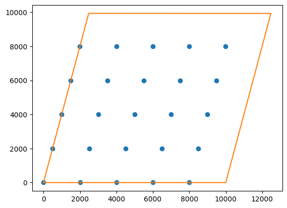
Quickly plotting the site boundary and initial position
[5]:
plt.plot(site.initial_position[:,0], site.initial_position[:,1], 'o')
ind = list(range(len(site.boundary))) + [0]
pt = plt.plot(site.boundary[ind,0], site.boundary[ind,1], '-')
Setting up the AEP calculator
Using the Gaussian wake model from Bastankhah & Porte Agel
Based on 16 wind direction to speed things up (not critical here because we will be using the RandomSearch algorithm)
[6]:
from py_wake.deficit_models.gaussian import IEA37SimpleBastankhahGaussian
from py_wake.aep_calculator import AEPCalculator

## We use the Gaussian wake model
wake_model = IEA37SimpleBastankhahGaussian(site, windTurbines)

## The AEP is calculated using n_wd wind directions
n_wd = 16
wind_directions = np.linspace(0., 360., n_wd, endpoint=False)

def aep_func(x, y, **kwargs):
    """A simple function that takes as input the x,y position of the turbines and return the AEP per turbine"""
    return wake_model(x=x, y=y, wd=wind_directions).aep().sum('wd').sum('ws').values*10**6
[7]:
#individual AEP per turbine
aep_func(site.initial_position[:,0], site.initial_position[:,1])
[7]:
array([48846666.47398125, 48076092.23666706, 47944165.03642996,
       47960611.08905267, 48321458.12536133, 48724302.1125211 ,
       47944055.20081887, 47677174.31239147, 47699818.49584734,
       48077384.1359745 , 48730772.05703812, 47956971.4742767 ,
       47746058.23357575, 47760605.9339205 , 48158379.95981343,
       48615025.49183208, 47864760.06397984, 47630113.20104554,
       47721845.464949  , 48135819.05773869, 48650994.84475809,
       47915433.78885604, 47687319.04146974, 47752944.44899338,
       48219457.74599594])
Setting up the NREL IRR cost model
Based on the 2006 NREL report (https://www.nrel.gov/docs/fy07osti/40566.pdf)
[8]:
from topfarm.cost_models.economic_models.turbine_cost import economic_evaluation as EE_NREL

def irr_nrel(aep, electrical_connection_cost, **kwargs):
    return EE_NREL(Drotor_vector, power_rated_vector, hub_height_vector, aep, electrical_connection_cost).calculate_irr()
Setting up the DTU IRR cost model
Based on Witold’s recent work
[9]:
from topfarm.cost_models.economic_models.dtu_wind_cm_main import economic_evaluation as EE_DTU

distance_from_shore = 10.0                               # [km]
energy_price = 0.2 / 7.4                                 # [DKK/kWh] / [DKK/EUR] -> [EUR/kWh]
project_duration = 20                                    # [years]
water_depth_array = 20 * np.ones([n_wt])                 # [m]
Power_rated_array = np.array(power_rated_vector)/1.0E3   # [MW]

ee_dtu = EE_DTU(distance_from_shore, energy_price, project_duration)

#setting up the IRR cost function
def irr_dtu(aep, electrical_connection_cost, **kwargs):
    ee_dtu.calculate_irr(
                    rated_rpm_array,
                    Drotor_vector,
                    Power_rated_array,
                    hub_height_vector,
                    water_depth_array,
                    aep,
                    electrical_connection_cost)
    return ee_dtu.IRR
Setting up the Topfarm problem
[10]:
#specify minimum spacing between turbines
min_spacing = 2 #@param {type:"slider", min:2, max:10, step:1}
#specify the cable cost
cable_cost_per_meter = 750. #@param {type:"slider", min:0, max:10000, step:1}
# Electrical grid cable components (Minimum spanning tree from Topfarm report 2010)
elnetlength = ElNetLength(n_wt=n_wt)
elnetcost = ElNetCost(n_wt=n_wt, output_key='electrical_connection_cost', cost_per_meter=cable_cost_per_meter)
# The Topfarm IRR cost model components
irr_dtu_comp = CostModelComponent(input_keys=[('aep',np.zeros(n_wt)), ('electrical_connection_cost', 0.0)],
n_wt=n_wt,
cost_function=irr_dtu,
output_keys="irr",
output_unit="%",
objective=True,
maximize=True)
irr_nrel_comp = CostModelComponent(input_keys=[('aep', np.zeros(n_wt)), ('electrical_connection_cost', 0.0)],
n_wt=n_wt,
cost_function=irr_nrel,
output_keys="irr",
output_unit="%",
objective=True,
maximize=True)
## User-defined cost model
irr_cost_models = {'DTU': irr_dtu_comp, 'NREL': irr_nrel_comp}
#select which IRR cost model to use
IRR_COST = 'DTU' #@param ["DTU", "NREL"]
# The Topfarm AEP component, returns an array of AEP per turbine
aep_comp = CostModelComponent(input_keys=['x','y'],
n_wt=n_wt,
cost_function=aep_func,
output_keys="aep",
output_unit="GWh",
objective=False,
output_vals=np.zeros(n_wt))
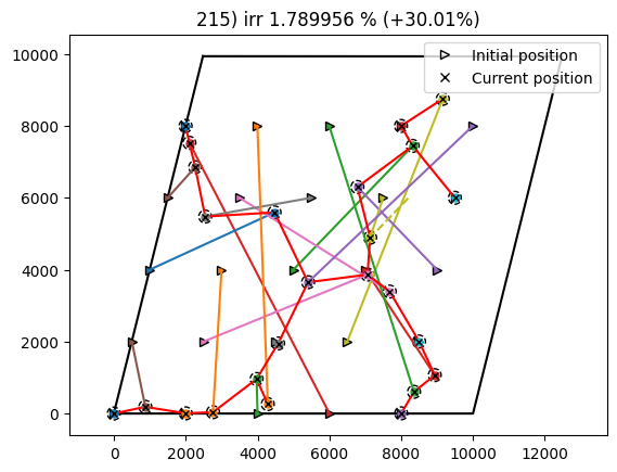
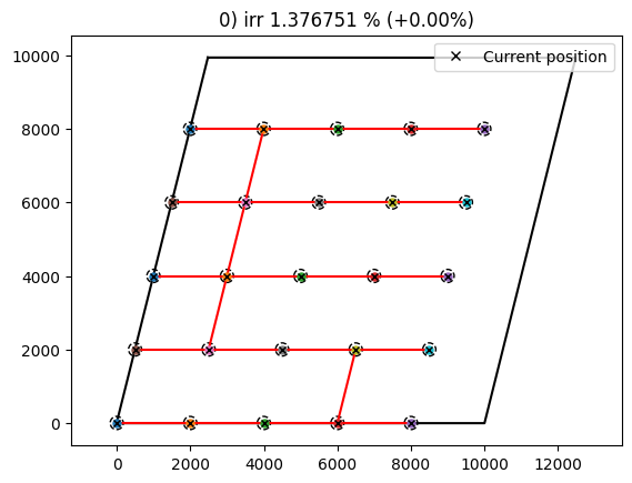
# Plotting component
plot_comp = XYCablePlotComp(memory=0, plot_improvements_only=False, plot_initial=False)
# The group containing all the components
group = TopFarmGroup([aep_comp, elnetlength, elnetcost, irr_cost_models[IRR_COST]])
problem = TopFarmProblem(
design_vars={'x':site.initial_position[:,0],
'y':site.initial_position[:,1]},
cost_comp=group,
n_wt = n_wt,
driver=EasyRandomSearchDriver(randomize_func=RandomizeTurbinePosition_Circle(), max_iter=100),
constraints=[SpacingConstraint(min_spacing * windTurbines.diameter(0)),
XYBoundaryConstraint(site.boundary)],
expected_cost=1.0,
plot_comp=plot_comp)
cost, state, recorder = problem.optimize()
INFO: checking out_of_order
INFO: checking system
INFO: checking solvers
INFO: checking dup_inputs
INFO: checking missing_recorders
INFO: checking unserializable_options
INFO: checking comp_has_no_outputs
INFO: checking auto_ivc_warnings
INFO: checking out_of_order
INFO: checking system
INFO: checking solvers
INFO: checking dup_inputs
INFO: checking missing_recorders
INFO: checking unserializable_options
INFO: checking comp_has_no_outputs
INFO: checking auto_ivc_warnings
C:\Users\mavar\Anaconda3\envs\topfarm\lib\site-packages\openmdao\core\group.py:1957: UnitsWarning:<model> <class Group>: Input 'cost_comp.comp_1.x' with units of 'm' is connected to output 'indeps.x' which has no units.
C:\Users\mavar\Anaconda3\envs\topfarm\lib\site-packages\openmdao\core\group.py:1957: UnitsWarning:<model> <class Group>: Input 'cost_comp.comp_1.y' with units of 'm' is connected to output 'indeps.y' which has no units.
Exercises
Try to see what is the effect of increasing or decreasing the cost of the cable
Change between IRR cost model. Ask Witold about the difference between DTU and NREL models