Layout Optimization with SGD driver

In this example, a layout optimization is performed with two different gradient-based drivers: Stochastic Gradient Descent (SGD) and Sequential Least Squares Quadratic Programming (SLSQP). The purpose is to draw a comparison between the two drivers in terms of accuracy in results and computational time.

Install TOPFARM if needed

# Install TopFarm if needed
import importlib
if not importlib.util.find_spec("topfarm"):
    !pip install git+https://gitlab.windenergy.dtu.dk/TOPFARM/TopFarm2.git

import numpy as np
import matplotlib.pyplot as plt
import time

We now import the site, wind turbine and wake models necessary to run the optimization.

from py_wake.deficit_models.gaussian import BastankhahGaussian
from py_wake.examples.data.lillgrund import LillgrundSite
from py_wake.utils.gradients import autograd
from py_wake.examples.data.hornsrev1 import HornsrevV80

We also import all the TOPFARM dependencies needed for the optimization.

from topfarm.cost_models.cost_model_wrappers import CostModelComponent
from topfarm.easy_drivers import EasySGDDriver, EasyScipyOptimizeDriver
from topfarm.plotting import XYPlotComp
from topfarm.constraint_components.spacing import SpacingConstraint
from topfarm import TopFarmProblem
from topfarm.constraint_components.boundary import XYBoundaryConstraint
from topfarm.recorders import TopFarmListRecorder
from topfarm.constraint_components.constraint_aggregation import ConstraintAggregation
from topfarm.constraint_components.constraint_aggregation import DistanceConstraintAggregation

Then we define the site, wind farm layout and wind resource. In this example, the turbine positions are created randomly and the wind resource is represented by the sector frequency as well as the Weibull A and k parameters.

# defining the site, wind turbines and wake model
site = LillgrundSite()
site.interp_method = 'linear'
windTurbines = HornsrevV80()
wake_model = BastankhahGaussian(site, windTurbines)

#wind farm layout
x_rows = 3 # 5 # (commented for speeding up notebook tests)
y_rows = 3 # 5
sgd_iterations = 100 # 2000
spacing = 3
xu, yu = (x_rows * spacing * windTurbines.diameter(), y_rows * spacing * windTurbines.diameter())
np.random.seed(4)
x = np.random.uniform(0, xu, x_rows * y_rows)
y = np.random.uniform(0, yu, x_rows * y_rows)
x0, y0 = (x.copy(), y.copy())
n_wt = x.size

#wind resource
dirs = np.arange(0, 360, 1) #wind directions
ws = np.arange(3, 25, 1) # wind speeds
freqs = site.local_wind(x, y, wd=dirs, ws=ws).Sector_frequency_ilk[0, :, 0]     #sector frequency
As = site.local_wind(x, y, wd=dirs, ws=ws).Weibull_A_ilk[0, :, 0]               #weibull A
ks = site.local_wind(x, y, wd=dirs, ws=ws).Weibull_k_ilk[0, :, 0]               #weibull k

The boundaries are set up as a simple rectangle enclosing the wind farm.

#boundaries
boundary = np.array([(0, 0), (xu, 0), (xu, yu), (0, yu)])

Now we set up the objective function and the gradient functions needed for the optimization for both drivers. The difference relies in the wind speed and wind direction samples. For the SGD driver, the wind speed and wind direction are generated randomly and follow a Weibull distribution. On the other hand, the SLSQP driver takes a user defined array of wind speed and wind directions to study.

# objective function and gradient function
samps = 50    #number of samples

#function to create the random sampling of wind speed and wind directions
def sampling():
    idx = np.random.choice(np.arange(dirs.size), samps, p=freqs)
    wd = dirs[idx]
    A = As[idx]
    k = ks[idx]
    ws = A * np.random.weibull(k)
    return wd, ws

#aep function - SGD
def aep_func(x, y, full=False, **kwargs):
    wd, ws = sampling()
    aep_sgd = wake_model(x, y, wd=wd, ws=ws, time=True).aep().sum().values * 1e6
    return aep_sgd

#gradient function - SGD
def aep_jac(x, y, **kwargs):
    wd, ws = sampling()
    jx, jy = wake_model.aep_gradients(gradient_method=autograd, wrt_arg=['x', 'y'], x=x, y=y, ws=ws, wd=wd, time=True)
    daep_sgd = np.array([np.atleast_2d(jx), np.atleast_2d(jy)]) * 1e6
    return daep_sgd

#aep function - SLSQP
def aep_func2(x, y, **kwargs):
    wd = np.arange(0, 360, 0.5)
    ws = np.arange(3, 25, 0.5)
    aep_slsqp = wake_model(x, y, wd=wd, ws=ws).aep().sum().values * 1e6
    return aep_slsqp

#gradient function - SLSQP
def aep_jac2(x, y, **kwargs):
    wd = np.arange(0, 360, 0.5)
    ws = np.arange(3, 25, 0.5)
    jx, jy = wake_model.aep_gradients(gradient_method=autograd, wrt_arg=['x', 'y'], x=x, y=y, ws=ws, wd=wd, time=False)
    daep_slsqp = np.array([np.atleast_2d(jx), np.atleast_2d(jy)]) * 1e6
    return daep_slsqp

We define the CostModelComponent which is responsible for evaluating the objective function and the gradients for the design variables selected.

#aep component - SGD
aep_comp = CostModelComponent(input_keys=['x','y'], n_wt=n_wt, cost_function=aep_func, objective=True, cost_gradient_function=aep_jac, maximize=True)

#aep component - SLSQP
aep_comp2 = CostModelComponent(input_keys=['x','y'], n_wt=n_wt, cost_function=aep_func2, objective=True, cost_gradient_function=aep_jac2, maximize=True)

cost_comps = [aep_comp2, aep_comp]

Next we set up the constraints for the problem. The constraints for the SGD driver are defined with the DistanceConstraintAggregation class.

Note: as the class is specified, the order of the SpacingConstraint and XYBoundaryConstraint must be kept as shown in this example.

min_spacing_m = 2 * windTurbines.diameter()  #minimum inter-turbine spacing in meters
constraint_comp = XYBoundaryConstraint(boundary, 'rectangle')

#constraints
constraints = [[SpacingConstraint(min_spacing_m), constraint_comp],
               DistanceConstraintAggregation([SpacingConstraint(min_spacing_m), constraint_comp],n_wt, min_spacing_m, windTurbines)]

Optimization with SGD driver

Some parameters need to be specified for the SGD driver such as max iterations, learning rate and the maximum time (in seconds). Only one optimization with a specific driver can be done at a time, which is defined by the driver_no variable.

#driver specs
driver_names = ['SLSQP', 'SGD']
drivers = [EasyScipyOptimizeDriver(maxiter=200, tol=1e-3),
           EasySGDDriver(maxiter=sgd_iterations, learning_rate=windTurbines.diameter()/5, max_time=18000, gamma_min_factor=0.1)]

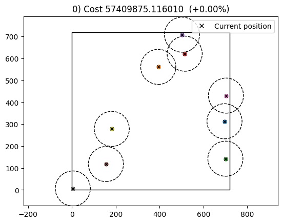
driver_no = 1    #SGD driver
ec = [10,1]      #expected cost for SLSQP (10) and SGD (1) drivers

Lastly we specify the TOPFARM problem.

tf = TopFarmProblem(
        design_vars = {'x':x0, 'y':y0},
        cost_comp = cost_comps[driver_no],
        constraints = constraints[driver_no],
        driver = drivers[driver_no],
        plot_comp = XYPlotComp(),
        expected_cost = ec[driver_no]
        )

INFO: checking out_of_order
INFO: checking system
INFO: checking solvers
INFO: checking dup_inputs
INFO: checking missing_recorders
INFO: checking unserializable_options
INFO: checking comp_has_no_outputs
INFO: checking auto_ivc_warnings

if 1:
    tic = time.time()
    cost, state, recorder = tf.optimize()
    toc = time.time()
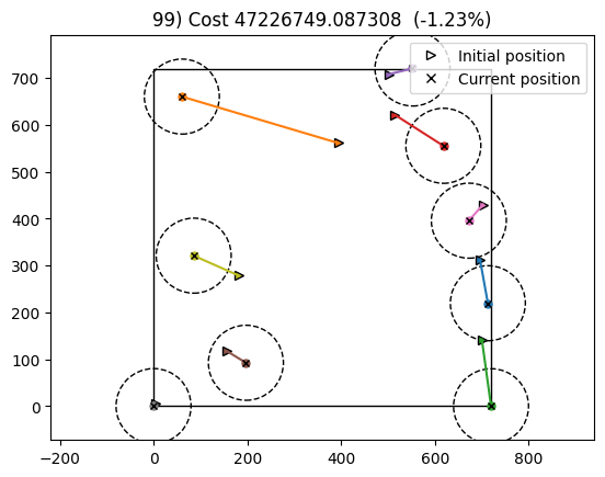
    print('Optimization with SGD took: {:.0f}s'.format(toc-tic), ' with a total constraint violation of ', recorder['sgd_constraint'][-1])
    recorder.save(f'{driver_names[driver_no]}')

INFO: checking out_of_order
INFO: checking system
INFO: checking solvers
INFO: checking dup_inputs
INFO: checking missing_recorders
INFO: checking unserializable_options
INFO: checking comp_has_no_outputs
INFO: checking auto_ivc_warnings

Optimization with SGD took: 8s  with a total constraint violation of  0.019866214451754457

Optimization with SLSQP driver

driver_no = 0                                     #SLSQP

tf = TopFarmProblem(
        design_vars = {'x':x0, 'y':y0},
        cost_comp = cost_comps[driver_no],
        constraints = constraints[driver_no],
        driver = drivers[driver_no],
        plot_comp = XYPlotComp(),
        expected_cost = ec[driver_no]
        )

if 1:
    tic = time.time()
    cost, state, recorder = tf.optimize()
    toc = time.time()
    print('Optimization with SLSQP took: {:.0f}s'.format(toc-tic))
    recorder.save(f'{driver_names[driver_no]}')

INFO: checking out_of_order
INFO: checking system
INFO: checking solvers
INFO: checking dup_inputs
INFO: checking missing_recorders
INFO: checking unserializable_options
INFO: checking comp_has_no_outputs
INFO: checking auto_ivc_warnings
INFO: checking out_of_order
INFO: checking system
INFO: checking solvers
INFO: checking dup_inputs
INFO: checking missing_recorders
INFO: checking unserializable_options
INFO: checking comp_has_no_outputs
INFO: checking auto_ivc_warnings

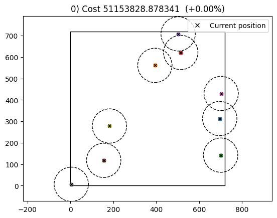
Optimization terminated successfully    (Exit mode 0)
            Current function value: -5576199.040992465
            Iterations: 18
            Function evaluations: 39
            Gradient evaluations: 18
Optimization Complete
-----------------------------------
Optimization with SLSQP took: 14s

Comparison between SGD and SLSQP driver performance

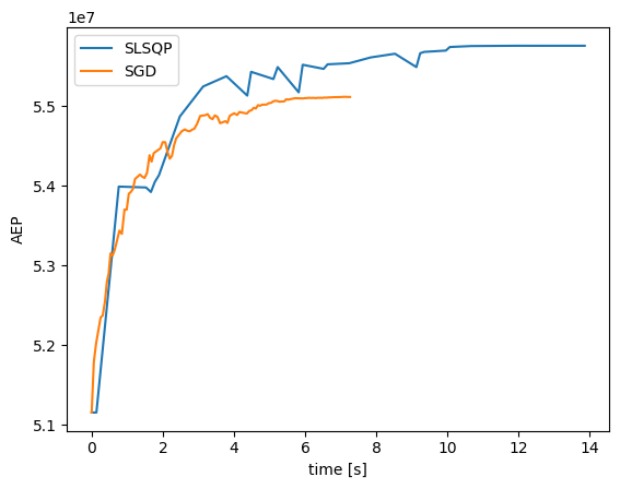
When we look into the optimization time for the SGD driver, we can see how the optimization took slightly less than the maximum time chosen of 180 seconds. In the case of the SLSQP driver, it is not known how much time the optimization will take, thus being able to set up a max_time proves advantageous. However, for more accurate results it is recommended to increase the maximum time.

We can also plot the AEP evolution in both cases to see the difference in terms of time and final optimized result. The AEP calculation for the SGD driver is re computed with the wind speed and wind direction distribution used for the SLSQP driver; that is, eliminating the random sampling introduced by the Monte Carlo approach.

if 1:
    plt.figure()
    for i in range(2):
        rec = TopFarmListRecorder().load(f'recordings/{driver_names[i]}')
        if driver_names[i] == 'SGD':
            aep = []
            for x, y in zip(rec['x'], rec['y']):
                aep.append(aep_func2(x, y))
            print('SGD AEP improvement: {:.2f}%'.format((aep[-1] - aep[0]) / aep[0] * 100))
        else:
            aep = rec['Cost']
            print('SLSQP AEP improvement: {:.2f}%'.format((aep[-1] - aep[0]) / aep[0] * 100))
        plt.plot(rec['timestamp']-rec['timestamp'][0], aep, label=driver_names[i])
    plt.legend()
    plt.xlabel('time [s]')
    plt.ylabel('AEP')

SLSQP AEP improvement: 9.01%
SGD AEP improvement: 7.75%

SGD Early Stopping

The SGD algorithm spends a fair amount of time treating constraint gradients as being more important than AEP gradients. The SGD algorithm can be sped up to turn off AEP computations after the learning rate has reached a specified fraction of the initial learning rate.

plt.plot(rec['timestamp']-rec['timestamp'][0], aep, label='Full SGD')
driver_no = 1
for early in [0.1, 0.05, 0.02]:

    constraints = [[SpacingConstraint(min_spacing_m), constraint_comp],
                   DistanceConstraintAggregation([SpacingConstraint(min_spacing_m), constraint_comp],n_wt, min_spacing_m, windTurbines)]
    #aep component - SGD
    aep_comp = CostModelComponent(input_keys=['x','y'], n_wt=n_wt, cost_function=aep_func, objective=True, cost_gradient_function=aep_jac, maximize=True)

    #aep component - SLSQP
    aep_comp2 = CostModelComponent(input_keys=['x','y'], n_wt=n_wt, cost_function=aep_func2, objective=True, cost_gradient_function=aep_jac2, maximize=True)

    cost_comps = [aep_comp2, aep_comp]

    tf = TopFarmProblem(
            design_vars = {'x':x0, 'y':y0},
            cost_comp = cost_comps[driver_no],
            constraints = constraints[driver_no],
            driver = EasySGDDriver(maxiter=sgd_iterations,
                                   learning_rate=windTurbines.diameter()/5,
                                   max_time=180000,
                                   gamma_min_factor=0.1, speedupSGD=True,
                                  sgd_thresh=early),
            plot_comp = None,
            expected_cost = ec[driver_no]
            )

    tic = time.time()
    cost, state, recorder = tf.optimize()
    toc = time.time()
    print('Optimization with SGD took: {:.0f}s'.format(toc-tic), ' with a total constraint violation of ', recorder['sgd_constraint'][-1])
    recorder.save(f'recordings/sgd_{early}')
    rec = TopFarmListRecorder().load(f'recordings/sgd_{early}')
    if recorder['sgd_constraint'][-1] > 1e-1: tag=' (invalid solution)'
    else: tag = ''
    aep = []
    for x, y in zip(rec['x'], rec['y']):
        aep.append(aep_func2(x, y))

    plt.plot(rec['timestamp'] - rec['timestamp'][0], aep, label=f'sgd_thresh={early}' + tag)

plt.legend()
plt.xlabel('time [s]')
plt.ylabel('AEP')

INFO: checking out_of_order
INFO: checking system
INFO: checking solvers
INFO: checking dup_inputs
INFO: checking missing_recorders
INFO: checking unserializable_options
INFO: checking comp_has_no_outputs
INFO: checking auto_ivc_warnings
INFO: checking out_of_order
INFO: checking system
INFO: checking solvers
INFO: checking dup_inputs
INFO: checking missing_recorders
INFO: checking unserializable_options
INFO: checking comp_has_no_outputs
INFO: checking auto_ivc_warnings
Optimization with SGD took: 2s  with a total constraint violation of  0.0
INFO: checking out_of_order
INFO: checking system
INFO: checking solvers
INFO: checking dup_inputs
INFO: checking missing_recorders
INFO: checking unserializable_options
INFO: checking comp_has_no_outputs
INFO: checking auto_ivc_warnings
INFO: checking out_of_order
INFO: checking system
INFO: checking solvers
INFO: checking dup_inputs
INFO: checking missing_recorders
INFO: checking unserializable_options
INFO: checking comp_has_no_outputs
INFO: checking auto_ivc_warnings
Optimization with SGD took: 3s  with a total constraint violation of  0.0
INFO: checking out_of_order
INFO: checking system
INFO: checking solvers
INFO: checking dup_inputs
INFO: checking missing_recorders
INFO: checking unserializable_options
INFO: checking comp_has_no_outputs
INFO: checking auto_ivc_warnings
INFO: checking out_of_order
INFO: checking system
INFO: checking solvers
INFO: checking dup_inputs
INFO: checking missing_recorders
INFO: checking unserializable_options
INFO: checking comp_has_no_outputs
INFO: checking auto_ivc_warnings
Optimization with SGD took: 3s  with a total constraint violation of  0.0

Text(0, 0.5, 'AEP')

# plot constraint violations

for early in np.flip([0.1, 0.05, 0.02]):
    rec = TopFarmListRecorder(f'./recordings/sgd_{early}.pkl')
    plt.plot(rec['sgd_constraint'], label=f'sgd_thresh={early}')

rec = TopFarmListRecorder(f'./recordings/SGD.pkl')
plt.plot(rec['sgd_constraint'], label=f'Full SGD', ls='--')
plt.xlabel('Iteration')
plt.ylabel("Constrain Violation $(m^2)$")
plt.yscale('log')
plt.legend()

<matplotlib.legend.Legend at 0x1c1f2d14640>